Accessing alerts via the Antares client

The alerts and additional properties about an object can be accessed via the various brokers’ API clients. This brief tutorial shows how to access alerts using the Antares client and Devkit. Other alert brokers have their own clients; consult their websites for documentation.

All of the following can be executed within a notebook in the RSP, or from a python prompt (or notebook) on your local computer.

Installing the client and devkit

Use pip to install the client and devkit by running the following on the command line (or, in a notebook cell, prepend a “!” for command-line access):

pip install --user antares_client
pip install --user antares_devkit

Retrieve an alert locus

Antares groups alerts and additional properties at a given position on the sky (i.e., associated with a particular astrophysical object) into an object called a “locus.” Each locus is given a unique ID in Antares. The following snippet will retrieve the locus for a known Antares ID. The locus is returned as a Python dict; the last line of this snippet prints the available dict keys. The lightcurve example below illustrates accessing the “alerts” entries in the dict; other items can be extracted in a similar way.

from antares_client import search
from antares_devkit.models import DevKitLocus

my_locus_id = "ANT2026z3bqyjga24oc"

locus_dict = search.get_by_id(my_locus_id).to_devkit(include_catalogs=True)

locus_dict.keys()

Plot a lightcurve from diaSource measurements

The following snippet extracts the flux measurements from the diaSource properties associated with each alert, then plots a lightcurve. Note that in the properties, negative fluxes are reported as positive values, but flagged with an “isNegative” flag. When plotting lightcurves, one should multiply fluxes with the “isNegative” flag by -1.

import matplotlib.pyplot as plt
import numpy as np

filter_colors = {'u': '#1600EA', 'g': '#31DE1F', 'r': '#B52626',
                 'i': '#370201', 'z': '#BA52FF', 'y': '#61A2B3'}
filter_names = list(filter_colors.keys())
filter_symbols = {'u': 'o', 'g': '^', 'r': 'v',
                  'i': 's', 'z': '*', 'y': 'p'}

temp_mjd = []
temp_band = []
temp_flux = []
for alert in locus_dict['alerts']:
    alert_id = str(alert['id'])
    if alert_id[0:4] == 'lsst':
        temp_mjd.append(alert['mjd'])
        temp_band.append(alert['properties']['lsst_diaSource_band'])
        if alert['properties']['lsst_diaSource_isNegative']:
            temp_flux.append(-1.0 * alert['properties']['lsst_diaSource_psfFlux'])
        else:
            temp_flux.append(alert['properties']['lsst_diaSource_psfFlux'])

mjd = np.asarray(temp_mjd, dtype='float')
band = np.asarray(temp_band, dtype='str')
flux = np.asarray(temp_flux, dtype='float')

fig = plt.figure(figsize=(6, 4))
for f, filt in enumerate(filter_names):
    fx = np.where(band == filt)[0]
    plt.plot(mjd[fx], flux[fx], filter_symbols[filt], color=filter_colors[filt], label=filt)
plt.xlabel('MJD')
plt.ylabel('PSF Flux [nJy]')
plt.legend(loc='upper right')
plt.title(my_locus_id)
plt.show()

The figure that is produced should look like the following:

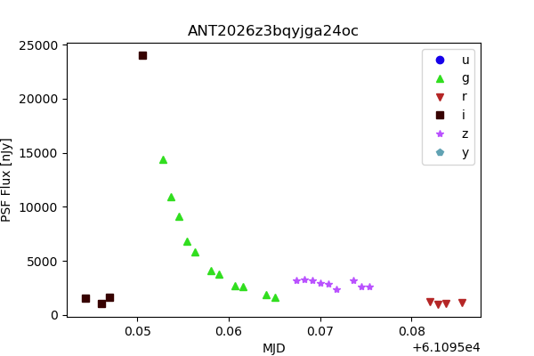
Figure 1: Lightcurve showing the flux measured on difference images as a function of time (in MJD) for a single Antares locus.